Data Source
The data displayed on this website and used for analysis was acquired from the United States Geological Survey (USGS) database. Surface water analysis was conducted on daily streamflow records, specifically daily mean flow rate given in cubic feet per second. The data used for the groundwater analysis was daily mean groundwater levels given in feet below the land surface. A select few of the sites provide only daily maximum and minimum water levels, and these were averaged in order to obtain an estimate of the daily mean water level. Due to the minimal daily variation of groundwater levels, this was deemed an adequate estimation. Several of the sites also provided measurements of water level above a specified datum, and data from those sites were converted into depth below land surface using the given elevation at the well location in order to normalize all of the groundwater data to create a uniform method for displaying the data. Metadata regarding the groundwater and surface water sites including latitude, longitude, elevation, aquifer (groundwater), and HUC/drainage area (surface water) was also retrieved from USGS.
Only data from the last water year plus the previous 29 water years was used for analysis for both groundwater and surface water. This cutoff was chosen in order to create a consistent analysis period (30 years) across sites to make the between site comparisons more equal. Groundwater wells and surface water sites were excluded from this analysis if they did not contain at least 300 daily mean values for at least 24 of the 30 years in question. Any records that did not include the day, month, and year of acquisition, were also removed.
Current State Metrics
The metrics chosen to represent the current state of Indiana groundwater were:
- Mean Water Table = Average annual value of daily mean water table depth,
- Maximum Water Table = Maximum annual value of the daily maximum water table depth,
- Minimum Water Table = Minimum annual value of the daily minimum water table depth,
- Water Table Range = Annual range of water table depth (defined as the Minimum annual water table depth minus the Maximum annual water table depth), and
- End of Year Water Table = The average water table depth on September 30th (the last day of the water year).
Metrics chosen to represent the current state of Indiana surface water resources are similar to those for groundwater, and are defined as follows:
- Mean Flow = Annual average value of daily discharge,
- Maximum Flow = Annual maximum value of daily discharge,
- Minimum Flow = Annual minimum value of 7-day mean discharge, and
- End of Year Flow = Daily discharge on September 30th (the last day of the water year).
Each of the above-mentioned parameters was calculated for each of the last 30 years of data. Annual metrics values were then sorted and ranked from smallest to largest. The non-exceedance probability (or percentile when multiplied by 100%) of the most recent water year was then calculated based on the previous 29 water years using the weibull plotting position (Weibull, 1951), which is similar to the method employed by the USGS for estimating percentiles (Helsel et al., 2020). The Weibull plotting position is given by:
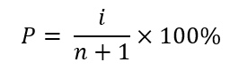
i = rank of the most year recent water year
n = number of years of data
Percentiles were only calculated for the End of Year metrics when no more than 6 values were missing for groundwater and surface water. Percentiles closer to 100% indicate a greater relative quantity of water present in the water year. For annual range, percentiles closer to 100% indicates a greater relative range in water levels for that year.
Results were then displayed geospatially using an ESRI ArcGIS web map, with symbology and color scales included with the maps. Additionally, graphs were created for each of the sites, where the daily values for the most recent year are plotted along with the mean value for the previous 29-years. This allows the user to visualize how the current year compares to previous years on a daily basis. The mean value was only plotted for days in which no more than 6 of the years contained missing data for that particular day.
Trend Analysis
Trends were evaluated for both the groundwater and surface data using the Mann-Kendall test (Kendall, 1975; Mann, 1945). The Mann-Kendall test was chosen, as it is a non-parametric, rank based test that is distribution free and not significantly affected by the presence of outliers. The Mann-Kendall test was used in a very similar trend analysis of Indiana surface waters (Kumar et al., 2009) as well as many other trend studies (Lettenmaier et al., 1994; Linns and Slack, 1999; Dixon et al., 2006).
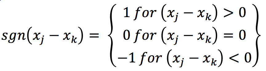
The Mann-Kendall test calculates an S statistic for a time series of length n with data points x1, x2, …, xn. The S statistic is given by:
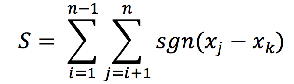
Where,
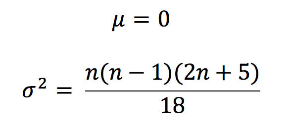
If no trend exists, then S follows a normal distribution centered on 0, where the mean and variance are given by:
To test for the significance of the test, the z test statistic is calculated and is given by:
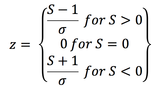
The z test statistic is used to calculate the probability of the trend existing. For this study, a significance level of α = 0.10 was used as a cutoff in determining if a statistically significant trend was present. The magnitude of the trends was determined using the Thiel-Sen slope estimator (β) (Sen, 1968; Thiel, 1950), which was used in a similar trend analysis (Kumar et al., 2009) and is also resistant to the effects of outliers. It is given by:
![]()
These results were then displayed geospatially using an ESRI ArcGIS web map. Layers were created to display the Thiel-Sen slope estiamte for all metrics. Map symbols also encode the results of the statistical trend test, to visualize which of the trends are statistically significant (p < .10).
References
Dixon, H., Lawler, D.M., Shamseldin, A.Y., 2006. Streamflow trends in western Britain. Geophysical Research Letters 33, L19406. doi:10.1029/2006GL027325.
Helsel, D.R., Hirsch, R.M., Ryberg, K.R., Archfield, S.A., and Gilroy, E.J., 2020, Statistical methods in water resources: U.S. Geological Survey Techniques and Methods, book 4, chap. A3, 458 p., https://doi.org/10.3133/tm4a3. [Super-sedes USGS Techniques of Water-Resources Investigations, book 4, chap. A3, version 1.1.]
Kendall, M.G., 1975. Rank Correlation Methods. Griffin, London.
Kumar, S., Merwade, V., Kam, J., Thurner, K., 2009. Streamflow trends in Indiana: Effects of long term persistence, precipitation, and subsurface drains. Journal of Hydrology 374, 171-183.
Lettenmaier, D.P., Wood, E.F., Wallis, J.R., 1994. Hydro-climatological trends in the continental United States, 1948–88. Journal of Climate 7 (4), 586–607.
Lins, H.F., Slack, J.R., 1999. Streamflow trends in the United States. Geophysical Research Letters 26 (2), 227–230.
Mann, H.B., 1945. Non-parametric tests against trend. Econometrica 13, 245–259.
Sen, P.K., 1968. Estimates of the regression coefficients based on Kendall’s tau. Journal of the American Statistical Association 63, 1379–1389.
Thiel, H., 1950. A rank-invariant method of linear and polynomial analysis, part 3. Netherlands Akademie van Wettenschappen, Proceedings 53, 1397–1412.
Weibull, W., 1951. A statistical distribution function for wide applicability. J. Applied Mechanics, 73, 293-297.